Bayesian House Edge

Frequentist p-values vs. Bayesian posterior probability

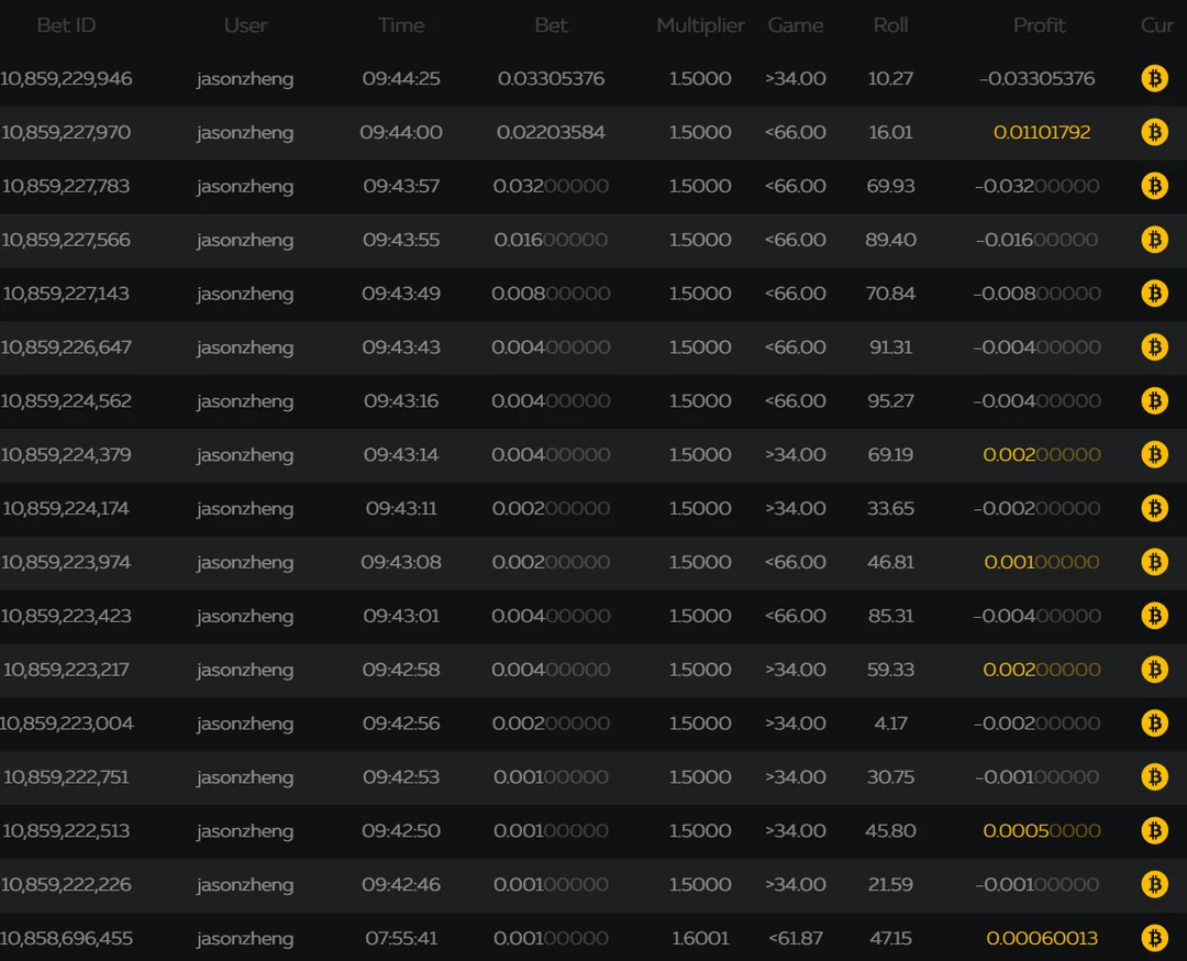
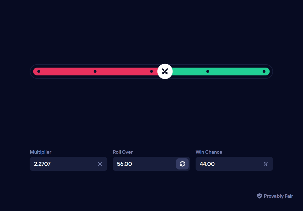
Most statistical audits lean on Frequentist hypothesis testing. The procedure assumes the casino is honest (the null hypothesis), then computes a p-value: the chance your losses happened through randomness alone. A p-value of 0.02 would trigger rejection of that hypothesis, and the audit would flag the game as rigged.

The problem: a p-value never answers what you actually want to know. You want the probability that the casino’s true house edge is worse than its claim. That question needs Bayesian statistics.

A Bayesian conjugate update fuses two inputs: your prior belief (the advertised edge plus how much you trust it) and your empirical data (wagers, net results, volatility). The output is an exact probability distribution for the true house edge — the real mathematical expectation behind the game. Our guide to Expected Value Explained covers why that distinction matters.

The math: Normal-Normal conjugate update

Over a large number of trials, your session results ($X$) approach a normal distribution by the Central Limit Theorem. That lets us model both the prior and the data as normal distributions and keep every step closed-form:

1. Defining the Prior (Claimed Edge)

Your belief about the house edge starts as a normal distribution:

Prior = N(μ_prior, σ²_prior)

Here $mu_{prior}$ is the claimed house edge, while $sigma^2_{prior}$ encodes your skepticism. Tight variance means you trust the operator; wide variance means you don’t.

2. Calculating the Data Likelihood

Your session produces an observed house edge ($mu_{data}$) with its own variance ($sigma^2_{data}$):

μ_data = -1 * Net_Profit / Total_Wagered
σ²_data = Volatility² / Total_Wagered

3. The Posterior Conjugate Update

The posterior for the true house edge is normal as well — the true mathematical expectation, $N(mu_{post}, sigma^2_{post})$, exactly as detailed in our guide to Expected Value Explained. The update runs as:

1 / σ²_post = 1 / σ²_prior + 1 / σ²_data
μ_post = σ²_post * (μ_prior / σ²_prior + μ_data / σ²_data)

Finally, the tool integrates that normal curve and reports the probability that the true edge exceeds twice the advertised claim:

P(True_Edge > 2 * Claimed_Edge) = 1 - Φ((2 * Claimed_Edge - μ_post) / σ_post)

Step-by-step audit: Auditing a slot claim

Take an online slot advertising a **2.00% house edge (98% RTP)** (the definitions sit in our guide on RTP vs House Edge). You run 10,000 spins at an average bet of $2 — $20,000 in total volume. The game’s standard deviation is 3.0. Your session ends $900 down, an observed loss rate of 4.50%.

1. Enter the claimed edge (2.00%) and set your prior confidence (e.g., standard prior variance).
2. Enter the session data: total wagers ($20,000), net result (-$900), and game volatility (3.0).
3. Click “Verify.” The auditor applies the Normal-Normal conjugate formulas.
4. Read the posterior curve. With a large losing sample, the posterior mean drifts toward 3.50%.
5. The output is a probability (e.g., 78%) that the slot’s true house edge beats the advertised figure — a single number quantifying possible operator manipulation.

Frequently asked questions